Welcome to pyodesys’s documentation!
Indices and tables
Overview


pyodesys provides a straightforward way
of numerically integrating systems of ordinary differential equations (initial value problems).
It unifies the interface of several libraries for performing the numerical integration as well as
several libraries for symbolic representation. It also provides a convenience class for
representing and integrating ODE systems defined by symbolic expressions, e.g. SymPy
expressions. This allows the user to write concise code and rely on pyodesys to handle the subtle differences
between libraries.
The numerical integration is performed using either:
Note that implicit steppers require a user supplied callback for calculating the Jacobian.
pyodesys.SymbolicSys derives the Jacobian automatically.
The symbolic representation is usually in the form of SymPy expressions, but the user may choose another symbolic back-end (see sym).
When performance is of utmost importance, e.g. in model fitting where results are needed
for a large set of initial conditions and parameters, the user may transparently
rely on compiled native code (classes in pyodesys.native.native_sys can generate optimal C++ code).
The major benefit is that there is no need to manually rewrite the corresponding expressions in another
programming language.
Documentation
Auto-generated API documentation for latest stable release is found here: https://bjodah.github.io/pyodesys/latest (and the development version for the current master branch is found here: http://hera.physchem.kth.se/~pyodesys/branches/master/html).
Installation
Simplest way to install pyodesys and its (optional) dependencies is to use the conda package manager:
$ conda install -c bjodah pyodesys pytest
$ python -m pytest --pyargs pyodesys
Optional dependencies
If you used conda to install pyodesys_ you can skip this section.
But if you use pip you may want to know that the default installation
of pyodesys only requires SciPy:
$ pip install pyodesys
$ pytest --pyargs pyodesys -rs
The above command should finish without errors but with some skipped tests. The reason for why some tests are skipped should be because missing optional solvers. To install the optional solvers you will first need to install third party libraries for the solvers and then their python bindings. The 3rd party requirements are as follows:
pygslodeiv2 (requires GSL >=1.16)
if you want to see what packages need to be installed on a Debian based system you may look at this Dockerfile.
If you manage to install all three external libraries you may install pyodesys with the option “all”:
$ pip install pyodesys[all]
$ pytest --pyargs pyodesys -rs
now there should be no skipped tests. If you try to install pyodesys on a machine where you do not have
root permissions you may find the flag --user helpful when using pip. Also if there are multiple
versions of python installed you may want to invoke python for an explicit version of python, e.g.:
$ python3.6 -m pip install --user pyodesys[all]
see setup.py for the exact list of requirements.
Using Docker
If you have Docker installed, you may use it to host a jupyter notebook server:
$ ./scripts/host-jupyter-using-docker.sh . 8888
the first time you run the command some dependencies will be downloaded. When the installation is complete there will be a link visible which you can open in your browser. You can also run the test suite using the same docker-image:
$ ./scripts/host-jupyter-using-docker.sh . 0
there will be one skipped test (due to symengine missing in this pip installed environment) and quite a few instances of RuntimeWarning.
Examples
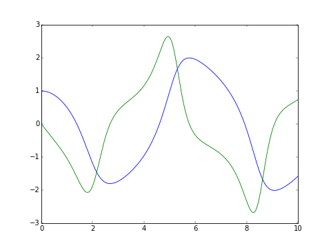
The classic van der Pol oscillator (see examples/van_der_pol.py)
>>> from pyodesys.symbolic import SymbolicSys
>>> def f(t, y, p):
...     return [y[1], -y[0] + p[0]*y[1]*(1 - y[0]**2)]
...
>>> odesys = SymbolicSys.from_callback(f, 2, 1)
>>> xout, yout, info = odesys.integrate(10, [1, 0], [1], integrator='odeint', nsteps=1000)
>>> _ = odesys.plot_result()
>>> import matplotlib.pyplot as plt; plt.show()
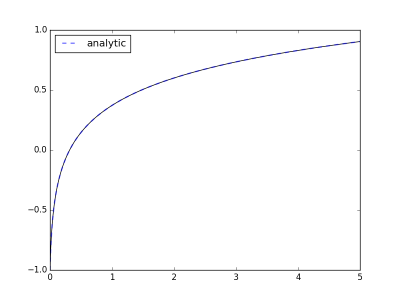
If the expression contains transcendental functions you will need to provide a backend keyword argument:
>>> import math
>>> def f(x, y, p, backend=math):
...     return [backend.exp(-p[0]*y[0])]  # analytic: y(x) := ln(kx + kc)/k
...
>>> odesys = SymbolicSys.from_callback(f, 1, 1)
>>> y0, k = -1, 3
>>> xout, yout, info = odesys.integrate(5, [y0], [k], integrator='cvode', method='bdf')
>>> _ = odesys.plot_result()
>>> import matplotlib.pyplot as plt
>>> import numpy as np
>>> c = 1./k*math.exp(k*y0)  # integration constant
>>> _ = plt.plot(xout, np.log(k*(xout+c))/k, '--', linewidth=2, alpha=.5, label='analytic')
>>> _ = plt.legend(loc='best'); plt.show()
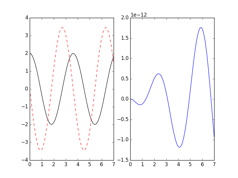
If you already have symbolic expressions created using e.g. SymPy you can create your system from those:
>>> import sympy as sp
>>> t, u, v, k  = sp.symbols('t u v k')
>>> dudt = v
>>> dvdt = -k*u  # differential equations for a harmonic oscillator
>>> odesys = SymbolicSys([(u, dudt), (v, dvdt)], t, [k])
>>> result = odesys.integrate(7, {u: 2, v: 0}, {k: 3}, integrator='gsl', method='rk8pd', atol=1e-11, rtol=1e-12)
>>> _ = plt.subplot(1, 2, 1)
>>> _ = result.plot()
>>> _ = plt.subplot(1, 2, 2)
>>> _ = plt.plot(result.xout, 2*np.cos(result.xout*3**0.5) - result.yout[:, 0])
>>> plt.show()
You can also refer to the dependent variables by name instead of index:
>>> odesys = SymbolicSys.from_callback(
...     lambda t, y, p: {
...         'x': -p['a']*y['x'],
...         'y': -p['b']*y['y'] + p['a']*y['x'],
...         'z': p['b']*y['y']
...     }, names='xyz', param_names='ab', dep_by_name=True, par_by_name=True)
...
>>> t, ic, pars = [42, 43, 44], {'x': 7, 'y': 5, 'z': 3}, {'a': [11, 17, 19], 'b': 13}
>>> for r, a in zip(odesys.integrate(t, ic, pars, integrator='cvode'), pars['a']):
...     assert np.allclose(r.named_dep('x'), 7*np.exp(-a*(r.xout - r.xout[0])))
...     print('%.2f ms ' % (r.info['time_cpu']*1e3))
...
10.54 ms
11.55 ms
11.06 ms
Note how we generated a list of results for each value of the parameter a. When using a class
from pyodesys.native.native_sys those integrations are run in separate threads (bag of tasks
parallelism):
>>> from pyodesys.native import native_sys
>>> native = native_sys['cvode'].from_other(odesys)
>>> for r, a in zip(native.integrate(t, ic, pars), pars['a']):
...     assert np.allclose(r.named_dep('x'), 7*np.exp(-a*(r.xout - r.xout[0])))
...     print('%.2f ms ' % (r.info['time_cpu']*1e3))
...
0.42 ms
0.43 ms
0.42 ms
For this small example we see a 20x (serial) speedup by using native code. Bigger systems often see 100x speedup.
Since the latter is run in parallel the (wall clock) time spent waiting for the results is in practice
further reduced by a factor equal to the number of cores of your CPU (number of threads used is set by
the environment variable ANYODE_NUM_THREADS).
For further examples, see examples/, and rendered jupyter notebooks here: http://hera.physchem.kth.se/~pyodesys/branches/master/examples
Run notebooks using binder
Using only a web-browser (and an internet connection) it is possible to explore the notebooks here: (by the courtesy of the people behind mybinder)
Citing
If you make use of pyodesys in e.g. academic work you may cite the following peer-reviewed publication:
Depending on what underlying solver you are using you should also cite the appropriate paper (you can look at the list of references in the JOSS article). If you need to reference, in addition to the paper, a specific point version of pyodesys (for e.g. reproducibility) you can get per-version DOIs from the zenodo archive:
Licenseing
The source code is Open Source and is released under the simplified 2-clause BSD license. See LICENSE for further details.
Contributing
Contributors are welcome to suggest improvements at https://github.com/bjodah/pyodesys (see further details here).